CUTLASS-Cute 初步(1)：Layout

github – Layout 测试代码

1. Layout

Cute(CUDA Tensor) 是 CUBLASS 扩展，用于简化张量 BLAS 操作和内存布局的管理。

最主要的概念是 Tensor 和 Layout：

Layout<Shape, Stride>: 定义张量的内存布局，用于将一维内存地址映射到多维张量索引。
- Shape：Logical dimensions，张量的逻辑维度/形状。
- Stride：Physical steps，每一个维度在内存中的步长/跨度。
Tensor<Engine,Layout>: 定义张量的数据类型/存储和布局。

映射公式：

offset = Σ (index[i] * stride[i])

Layout 本质是一个映射函数，将多维索引映射到一维内存地址。称索引为定义域(domain)，映射得到的地址为值域(codomain)。以一个一维映射为例：

1d_map_stirde2

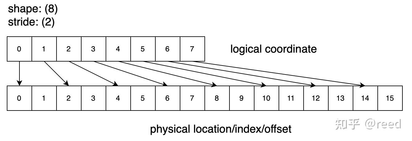
如上图 layout (8):(2)，按照映射公式得到 index_phy = index_logic * 2，将连续以一维索引 0,1,2,…7 映射到内存地址 0,2,4,…14。此时：

size(layout) = 8
cosize(layout) = 16

而如果定义 layout (8):(0)，则所有逻辑索引都映射到内存地址偏移 0，即所有索引映射到同一个地址。此时得到：

size(layout) = 8
cosize(layout) = 1

1.1. CuTe IntTuple

定义多维 Tensor 时，可以使用嵌套的 Shape 和 Stride 来定义子 Tensor 的形状和步长。在 Cute 中，使用 template tuple 表示表示嵌套的 Shape 和 Stride。

具体是使用 IntTule 表示：IntTuple 可以是一个整形，也可以是一个 tuple，并且可以嵌套。以下都是一个合法的 IntTuple：

int{3}，运行时整数。
Int<3>{}，Int<3>() 编译时整数，称为静态整数。另外，定义了一些字面量：比如 _1、_2、_3 分别定义为 Int<1>{}、Int<2>{}、Int<3>{}。
带有任何模板参数的 IntTuple，比如 make_tuple(int{2}, Int<3>{})。

在对 layout 进行一些操作时，还定义了一些常量表示这些操作：

cute::_ : 获取 slice 时，表示或者这个维度（轴）的所有数据，在 Python 中类似于 :。
cute::X ：在切分操作（比如 partition 操作）的时候，表示不对这个维度进行切分。

1.2. rank 和 depth

Rank 只看最外层有几个元素，不管里面嵌套了什么。一些 layout 示例 rank：

Layout Shape        rank    含义
────────────        ────    ────
(8)                 1       向量（1 个 mode）
(4,2)               2       矩阵（2 个 mode：行和列）
(M,N,K)             3       3-D tensor（3 个 mode）
((2,2),2)           2       还是矩阵！虽然内部有嵌套，顶层只有 2 个 mode

Depth 度量的是括号嵌套的深度，一些示例：

IntTuple              depth    解释
────────              ─────    ────
6                     0        没有括号，就是个整数
(4,3)                 1        一层括号
(3,(6,2),8)           2        最深处 (6,2) 嵌套了 2 层
((2,(1,3)),4)         3        最深处 (1,3) 嵌套了 3 层

2. Layout 示例

2.1. 例一：定义一个两行三列的矩阵布局，这个矩阵采用列主序存储

    auto tensor_shape = make_shape(2, 3);   // 两行三列
    auto tensor_stride = make_stride(1, 2); // 列主序存储
    auto tensor_layout = make_layout(tensor_shape, tensor_stride);
    print_layout(tensor_layout);

输出：

(2,3):(1,2)
      0   1   2
    +---+---+---+
 0  | 0 | 2 | 4 |
    +---+---+---+
 1  | 1 | 3 | 5 |
    +---+---+---+

// A(m, n) = storage[m*1 + n*2]
const auto val = tensor_layout(1, 2); // 访问张量元素 (1,2)，值为 5

2.2. 例二：定义一个两行三列的矩阵，这个矩阵采用行主序存储

    auto tensor_shape = make_shape(2, 3);   // 两行三列
    auto tensor_stride = make_stride(3, 1); // 行主序存储
    auto tensor_layout = make_layout(tensor_shape, tensor_stride);
    print_layout(tensor_layout);

输出：

(2,3):(3,1)
      0   1   2
    +---+---+---+
 0  | 0 | 1 | 2 |
    +---+---+---+
 1  | 3 | 4 | 5 |
    +---+---+---+

2.3. 例三：定义一个三维张量布局

张量形状：(4,2,2)，dim0=4, dim1=2, dim2=2
张量步长：(4,1,2) 行主序存储，子 tensor 为列主序

    auto tensor_shape = make_shape(4, make_shape(2, 2));
    auto tensor_stride = make_stride(4, make_stride(1, 2));
    auto tensor_layout = make_layout(tensor_shape, tensor_stride);
    print_layout(tensor_layout);

输出：

    (4,(2,2)):(4,(1,2))
           0    1    2    3
        +----+----+----+----+
     0  |  0 |  1 |  2 |  3 |
        +----+----+----+----+
     1  |  4 |  5 |  6 |  7 |
        +----+----+----+----+
     2  |  8 |  9 | 10 | 11 |
        +----+----+----+----+
     3  | 12 | 13 | 14 | 15 |
        +----+----+----+----+

// A(i, (j, k)) = storage[i*4 + j*1 + k*2]
const auto val1 = tensor_layout(2, make_coord(1, 0)); // 访问张量元素 (2,(1,0))，值为 9

2.4. 例四：定义一个三维张量布局

张量形状：(4,2,2)，dim0=4, dim1=2, dim2=2
张量步长：(2,1,8)

    auto tensor_shape = make_shape(4, make_shape(2, 2));
    auto tensor_stride = make_stride(2, make_stride(1, 8));
    auto tensor_layout = make_layout(tensor_shape, tensor_stride);
    print_layout(tensor_layout);

输出：

    (4,(2,2)):(2,(1,8))
           0    1    2    3
        +----+----+----+----+
     0  |  0 |  1 |  8 |  9 |
        +----+----+----+----+
     1  |  2 |  3 | 10 | 11 |
        +----+----+----+----+
     2  |  4 |  5 | 12 | 13 |
        +----+----+----+----+
     3  |  6 |  7 | 14 | 15 |
        +----+----+----+----+

// A(i, (j, k)) = storage[i*2 + j*1 + k*8]
const auto val1 = tensor_layout(2, make_coord(1, 0)); // 访问张量元素 (2,(1,0))，值为 5

几何解释：

内存布局（一维）：
[0][1][2][3][4][5][6][7] | [8][9][10][11][12][13][14][15]
 ←───── 块 k=0 ─────→     ←────── 块 k=1 ──────→

Stride 分量	值	含义
stride_i	2	沿 i 方向移动一步，offset 增加 2
stride_j	1	沿 j 方向移动一步，offset 增加 1
stride_k	8	沿 k 方向移动一步，offset 增加 8（跳到另一个块）

关于几何解释，更多理解内容参考帖子 https://note.gopoux.cc/hpc/cute/layout/

3. Hierarchy Layout

层级化的 layout 概念用于更加直观的表示多维 tensor，拆分 layout 划分工作，更好的表示内存局部性，如 TV layout。

hierarchy_layout

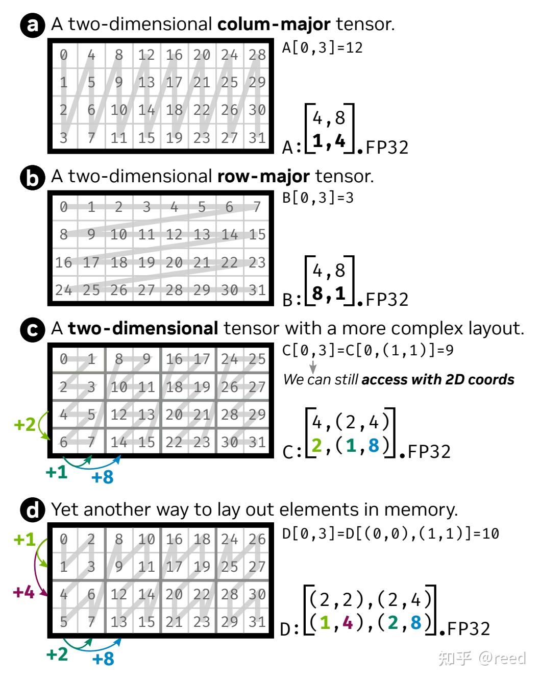
上图示例中，a, b 情形分别表示 column-major 和 row-major 布局的二维矩阵，不存在嵌套。

3.1. 嵌套 layout 示例 c

layout_424_218

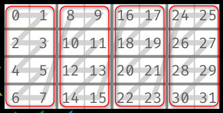
示例 c 中，可以将其看作一个嵌套的 layout：在列方向上存在一个嵌套的 layout。

内层 layout （红色框内）为: (4, 2):(2, 1)。
外层 layout 为: (1, 4):(4, 1)。即外层 layout 是一个有 1 行 4 列的矩阵（向量），每个元素是一个内层 layout。

合并之后，表示 4 行 8 列。其中，列方向为两个层次：(2, 4)，2 表示内层 layout 的列数，4 表示外层 layout 的列数。

综合起来的 shape 为 (4, (2, 4))，其含义为（按顺序表示）：第一个 4 表示行数，2 表示内层 layout 列数，第二个 4 表示外层 layout 列数。

针对 stride，其表示顺序要与 shape 保持一致，即如果 shape 为 (sx, (sy, sz))，则 stride 为 (dx, (dy, dz))即 stride(2, (1, 8)) 的含义如下：

dx：内层 layout 行方向的间隔为 2。注意：这里解读为内层 layout 的行方向间隔，这个 layout 在行方向上没有外层。
dy：内层 layout 列方向的间隔为 1。
dz：外层 layout 列方向的间隔为 8，即为一个内层 layout 块的大小。

综合得到 layout 为 (4, (2, 4)):(2, (1, 8))。

3.2. 嵌套 layout 示例 d

layout_424_128

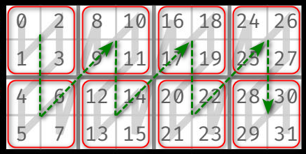
示例 d 的 layout 在行列方向上均存在嵌套 layout。两层 layout 分别为：

内层 layout （红色框内）为: (2, 2):(2, 2)。
外层 layout 为: (2, 4):(4, 1)。

合并之后，表示 4 行 8 列。其中，行方向为两个层次：(2, 2)，列方向为两个层次：(2, 4)。即：

((sx1, sx2):(sy1, sy2))，得到综合 shape 为 ((2, 2), (2, 4))。
- sx1 表示内层 layout 行数，sx2 表示外层 layout 行数；
- sy1 表示内层 layout 列数，sy2 表示外层 layout 列数。
对应的，综合 stride 为 ((dx1, dx2), (dy1, dy2))，得到((1, 4), (2, 8))。

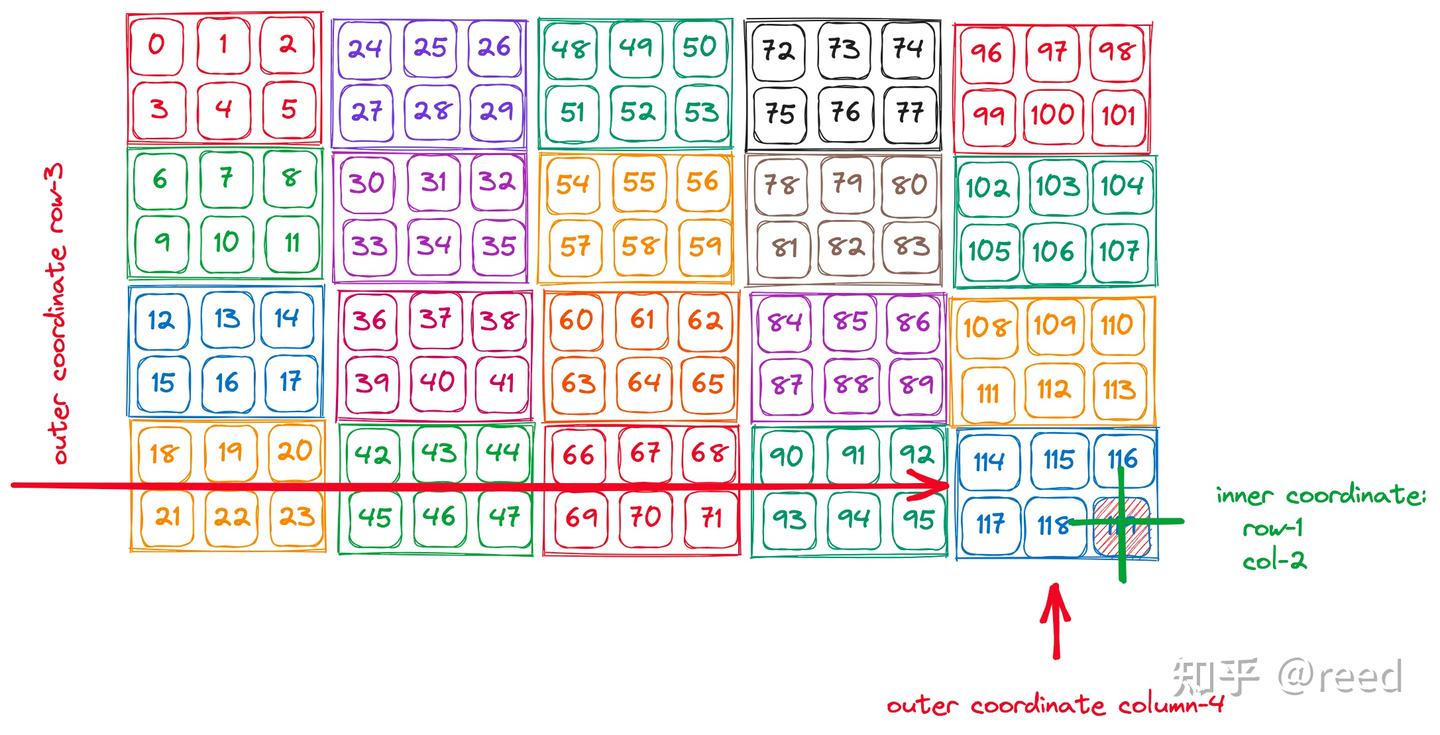
3.3. 坐标及数据访问 coordinate

对一个 layout 为 ((2, 4), (3, 5)):((3, 6), (1, 24)) 的 tensor 进行数据访问时，其访问格式遵从上述的顺序，形式为：

auto row_coord = make_coord(1, 3);
auto col_coord = make_coord(2, 4);
auto coord = make_coord(row_coord, col_coord);

如下图所示：

hierarchy_layout_coord

3.4. slice 操作

CuTe 提供了 slice 函数，使用 UnderScore cute::_，用于获取指定维度的子 layout。如下图所示：

hierarchy_layout_slice

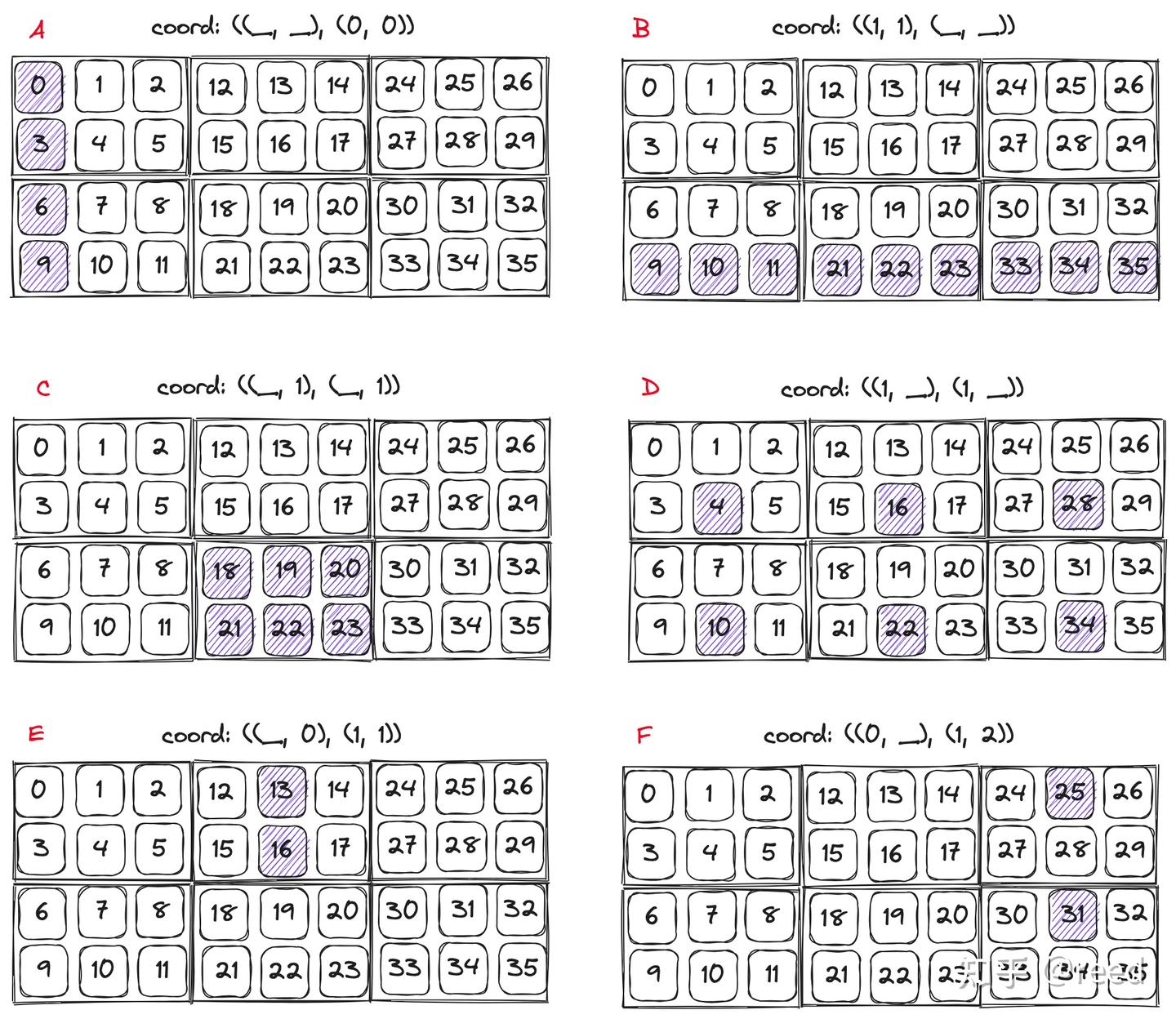
使用方式如下：

auto layout = make_layout(
    make_shape(make_shape(2, 4), make_shape(3, 5)),
    make_stride(make_stride(3, 6), make_stride(1, 24))
);

auto row_coord = make_coord(1, 1);
auto col_coord = make_coord(cute::_, cute::_);
auto coord = make_coord(row_coord, col_coord); // 获取子块 B
auto sub_layout = cute::slice(coord, layout);

4. Layout compatibility 以及 coordinate 转换

一个 layout，都有三个坐标空间，即不同的索引方式：

1-D
R-D：rank-D，即多维索引方式。
h-D：hierarchy-D，即层级化索引方式，也叫 natural 方式。

转换的原则是 layout 兼容，即 layout compatible。当其 shape 兼容另一个 layout 的 shape 时，两个 layout 兼容。对于 compatible 的 layout，可以进行 coordinate 转换。兼容的条件：

size(layout1) == size(layout2)
layout1 中的所有坐标都可以用作 layout2 的坐标，即 layout1 的定义域包含于 layout2 的定义域。

4.1. 坐标转换

Cute 使用余字典序（colexicographical order）对输入坐标转换为 natural 坐标，即左侧的维度（轴）变化更快。以 shape(3, (2, 3)) 为例：

1-D	2-D	Natural	1-D	2-D	Natural
`0`	`(0,0)`	`(0,(0,0))`	`9`	`(0,3)`	`(0,(1,1))`
`1`	`(1,0)`	`(1,(0,0))`	`10`	`(1,3)`	`(1,(1,1))`
`2`	`(2,0)`	`(2,(0,0))`	`11`	`(2,3)`	`(2,(1,1))`
`3`	`(0,1)`	`(0,(1,0))`	`12`	`(0,4)`	`(0,(0,2))`
`4`	`(1,1)`	`(1,(1,0))`	`13`	`(1,4)`	`(1,(0,2))`
`5`	`(2,1)`	`(2,(1,0))`	`14`	`(2,4)`	`(2,(0,2))`
`6`	`(0,2)`	`(0,(0,1))`	`15`	`(0,5)`	`(0,(1,2))`
`7`	`(1,2)`	`(1,(0,1))`	`16`	`(1,5)`	`(1,(1,2))`
`8`	`(2,2)`	`(2,(0,1))`	`17`	`(2,5)`	`(2,(1,2))`

其转换方法为：对整数做从左到右的逐级取模和除法：

以二维 layout (M，N) 为例，从 1-D 转换到 2-D 的方法如下：

coord = (index % M, (index / M) % N)

以三维 layout (M, (N, K)) 为例，从 1-D 转换到 h-D 的方法如下：

coord = (index % M, ((index / M) % N, (index / (M*N)) % K))

三维 index -> coord 具体示例：

i = 7 为例：
  第一维大小 = 3:   7 % 3 = 1,  7 / 3 = 2
  第二维是 (2,3)：
    子维度大小 = 2:  2 % 2 = 0,  2 / 2 = 1
    子维度大小 = 3:  1 % 3 = 1

结果: (1, (0, 1))

使用 cute::idx2crd(idx, shape) 转换的时候，就是使用 colex order 来进行转换的：

        idx2crd                          crd2idx
1-D ──────────→ natural (h-D) coord ──────────→ index
                     ↑
        idx2crd      │
R-D ──────────→──────┘

转换示例：

auto shape = Shape<_3,Shape<_2,_3>>{};
print(idx2crd(   16, shape));                                // (1,(1,2))
print(idx2crd(_16{}, shape));                                // (_1,(_1,_2))
print(idx2crd(make_coord(   1,5), shape));                   // (1,(1,2))
print(idx2crd(make_coord(_1{},5), shape));                   // (_1,(1,2))
print(idx2crd(make_coord(   1,make_coord(1,   2)), shape));  // (1,(1,2))
print(idx2crd(make_coord(_1{},make_coord(1,_2{})), shape));  // (_1,(1,_2))

对一个 layout，使用这三种坐标索引方式，无论使用哪种坐标去调用 layout(…)，只要指的是同一个逻辑位置，得到的 index 完全相同。

cute::Layout 提供两种映射。从输入坐标转换为 natural 坐标时，与 stride无关。使用 layout 映射计算得到 index 时，则需要使用各维度的 stride。总结如下表：

操作	依赖 Shape	依赖 Stride
1-D ↔ R-D ↔ h-D 坐标转换 (idx2crd)	✅	❌
坐标兼容性判断 (compatibility)	✅	❌
坐标 → 内存 index (crd2idx)	✅	✅

4.2. LayoutLeft 和 LayoutRight

使用 cute::make_layout 创建一个 layout 时，如果不指定 stride，则使用 LayoutLeft 的方式生成 stride，即紧凑列主序：

Layout s2xh4 = make_layout(make_shape(2, make_shape(2, 2)), make_stride(4, make_stride(2, 1)));
Layout s2xh4_col = make_layout(shape(s2xh4), LayoutLeft{});
print_layout(s2xh4_col);

打印 layout 如下：

(2,(2,2)):(_1,(2,4))
      0   1   2   3
    +---+---+---+---+
 0  | 0 | 2 | 4 | 6 |
    +---+---+---+---+
 1  | 1 | 3 | 5 | 7 |
    +---+---+---+---+

LayoutLeft、colexicographical order、column-major 都是指同一种布局方式，即列主序。

参考及资料

reed – cute 之 Layout
Yifan Yang (杨轶凡) – CuTe Layout and Tensor
CUTLASS CUTE 1 Layout Algebra
01_layout.md：CUTLASS/CuTe 官方文档