CUTLASS-Cute 初步(2):Tensor & Layout Algebra
0. 紧凑 stride 的生成:LayoutLeft 与 LayoutRight
当调用 make_layout(shape) 而不显式指定 stride 时,CuTe 使用 LayoutLeft(紧凑列主序)自动生成 stride。也可以通过 LayoutRight(紧凑行主序)来构造。
auto shape = make_shape(2, make_shape(2, 2));
auto manual = make_layout(shape, make_stride(4, make_stride(2, 1)));
auto left   = make_layout(shape, LayoutLeft{});   // 等价
auto right  = make_layout(shape, LayoutRight{});
print_layout(left);
print_layout(right);
LayoutLeft 生成 stride 的算法是”从左侧开始的 exclusive prefix product”——shape 从左到右做前缀乘,得到广义列主序 stride:
(2,(2,2)):(_1,(2,4))
      0   1   2   3
    +---+---+---+---+
 0  | 0 | 2 | 4 | 6 |
    +---+---+---+---+
 1  | 1 | 3 | 5 | 7 |
    +---+---+---+---+
LayoutRight 从右侧开始做 exclusive prefix product,对于 depth=1 的 shape 就是行主序,但对层级 shape 的结果可能不符合直觉。
LayoutLeft、colexicographical order、column-major 本质上对应同一种遍历顺序(列优先)。LayoutRight 则对应 row-major。
理解 stride 是如何自动生成的,有助于理解后面的 coalesce 和 composition 操作为什么会有特定的行为。
1. CuTe 中的 Tensor 划分 (Partitioning a Tensor)
在 GEMM 计算是,需要对矩阵进行划分(分块),以便线程块(Thread Block)和线程(Thread)能够并行处理数据。常用的有 Inner-Partitioning、Outer-Partitioning,以及 TV-layout-Partition。
1.1. Inner-Partitioning
GEMM 计算,先需要按照 Thread Block 划分为若干 Tile,即给每个 Thread Block 分配一个 Tile。如下所示:
Tensor A = make_tensor(ptr, make_shape(8,24));  // (8,24)
auto tiler = Shape<_4,_8>{};                    // (_4,_8)

Tensor tiled_a = zipped_divide(A, tiler);       // ((_4,_8),(2,3))
在使用 tiler 对 A 进行切分之后,(_4, _8) 是第一个mode(first mode),(2, 3) 是第二个mode(second mode)。
- 第一个 mode (mode 0):Tile 的 shape
- 第二个 mode (mode 1):Tile 在全局中的排列
mode 是
张量代数(tensor algebra)中的一个概念,表示张量的不同维度,或者叫逻辑轴。为了避免与 tensor 中的维度(dimension)混淆,故使用不同的术语。
沿着第二个mode 切分之后,可以得到 2x3 个 Tile,每个 Tile 的 shape 是 4x8:
Tensor cta_a = tiled_a(make_coord(_,_), make_coord(blockIdx.x, blockIdx.y)); // (_4,_8)
由于保留了内部 tile 的 shape 信息,这种切分方式叫做 Inner-Partitioning。CuTe 使用 inner_partition(Tensor, Tiler, Coord) 函数来实现内部分块,在实际使用时,则使用另外一个代替的函数 local_tile(Tensor, Tiler, Coord)来进行 tile 划分(分配给 Thread Block)。
1.2. Outer-Partitioning
在 Thread Block 划分好 tile 之后,下一步就是将 sub-tile 分配给线程(Thread):
Tensor thr_a = tiled_a(threadIdx.x, make_coord(_,_)); // (2,3)
这一步叫做 Outer-Partitioning,因为这种划分方式对 tile 进行划分,保留了分块的 shape 信息。在 CuTe 中,使用 outer_partition(Tensor, Tiler, Coord) 函数来实现外部分块,在实际使用时,则使用另外一个代替的函数 local_partition(Tensor, Layout, Idx) 来进行 sub-tile 划分(分配给 Thread)。
2. Layout Algebra
2.1. Coalesce:Layout 展平为一维
一些二维的 layout,其二维索引 (m, n) 可以转换得到对应的一维索引 k。例如:
layout (M, N) : (1, M)
k = m + n * M
例子:
auto layout = Layout<Shape<_2,Shape <_1,_6>>,
                     Stride<_1,Stride<_6,_2>>>{};
auto result = coalesce(layout);    // _12:_1
有三种情况可以展平:
- (s0, _1) : (d0, d1) => s0 * d0。忽略第二维的 stride。
- (_1, s1) : (d0, d1) => s1 * d1。忽略第一维的 stride。
- (s0, s1) : (d0, d1) => s0 + s1 * d0。当 d1 == d0 * s0 时,可以展平为一维。
其他情况不能展平为一维 layout,比如 layout codomain 出现空洞,即不是连续映射的。不能展平的维度维持原有的 shape 和 stride 信息。
在 CuTe 中,以一个二维 layout 为例,可以使用layout(m, n) 索引的形式访问,也可以使用 layout(k) 的形式访问。使用一维索引 k 访问时,其应该等于使用 coalesce 展平后的 layout 进行访问。见https://github.com/NVIDIA/cutlass/blob/main/test/unit/cute/core/coalesce.cpp。
2.1.1. By-mode Coalesce:展平部分轴
例如 layout ((M, N), K, L) : ((1, M), M * N, M * N * K),希望展平子 layout (M, N):(1, M),保持其他轴的 shape 不变:
coalesce(layout, Step<_1, _1, _1>{});
Step<_1, _1, _1> 表示展平为三维的 layout,因为这个 Step<> 的 rank 是 3。CuTe 对每个轴重新计算,得到新的 layout:
((M*N), K, L) : (1, M*N, M*N*K)
一个完整的例子:
// Coalesce within each top-level mode
auto layout = make_layout(make_shape(Int<2>{}, make_shape(Int<1>{}, Int<6>{})),
                          make_stride(Int<1>{}, make_stride(Int<6>{}, Int<2>{})));
// layout is (2,(1,6)):(1,(6,2))

auto result = coalesce(layout, Step<_1,_1>{});  // result is (2,6):(1,2)
// Coalesced within each mode, preserving rank-2 structure
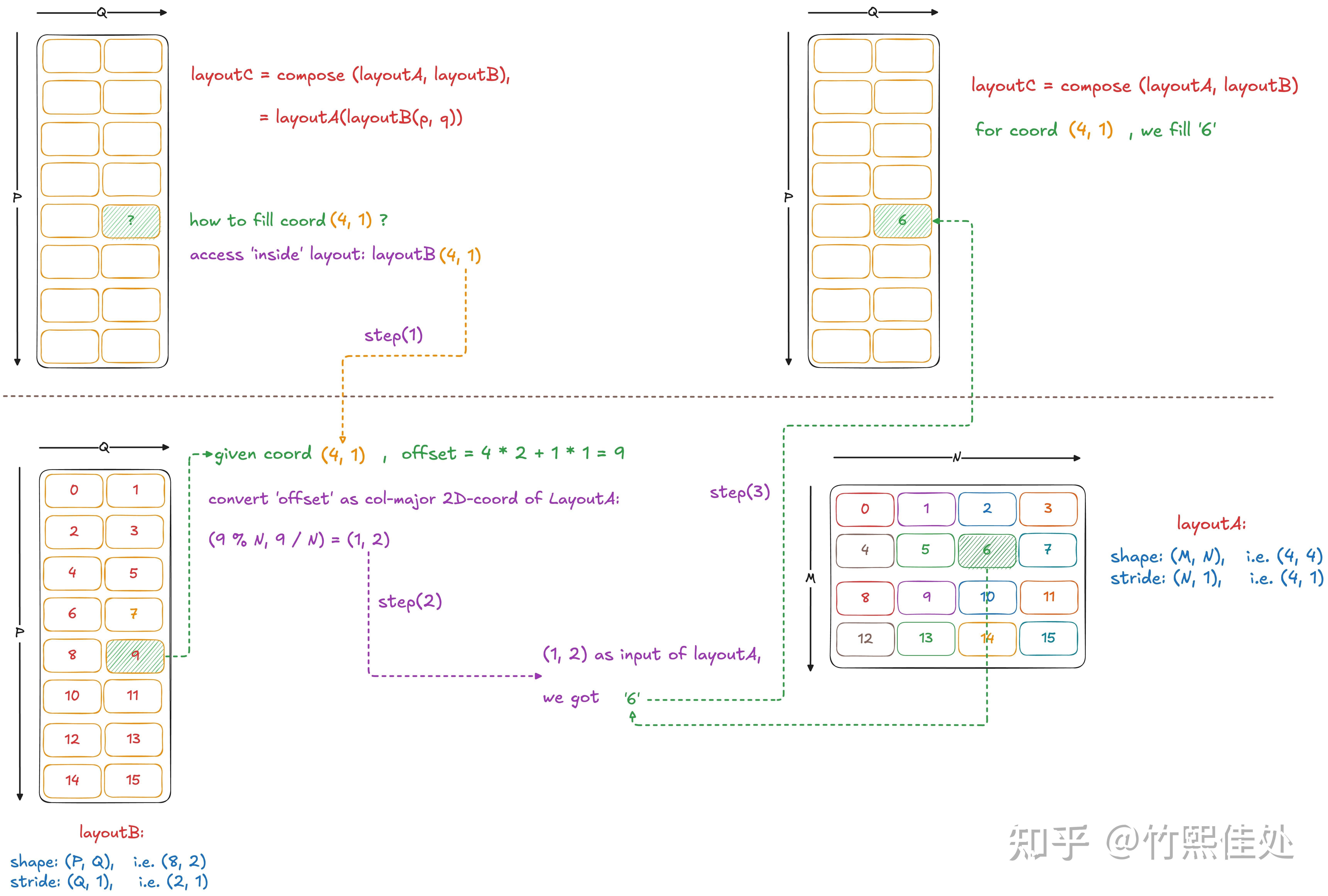
2.2. Composition:Layout 复合
首先,Layout 本质就是一个映射函数,Composition 即经过多次映射:
R(c) := (A o B)(c) := A(B(c))
计算过程如下:
composition 有如下属性:
- 兼容性:compatible(B, R) - B的每个坐标都可以用作R的坐标,因为B定义了R的定义域
- 函数等价性:对于B定义域内的所有i,R(i) == A(B(i))。官方测试用例test composition
2.2.1. By-mode Composition
composition 函数提供一个重载版本,第二个参数为 tiler,对部分维度(轴)进行复合操作。Tiler 可以是:
- 一个 Layout
- Tiler tuple
- Shape,会被解释为步长为 1 的 Tiler
2.2.2. Composition:reshape & reordering
Reshape
// 20-element layout with stride 2
auto layout_1d = make_layout(Int<20>{}, Int<2>{});  // 20:2

// Reshape to 5x4 row-major
auto tiler = make_layout(make_shape(Int<5>{}, Int<4>{}),
                         make_stride(Int<4>{}, Int<1>{}));  // (5,4):(4,1)

auto result = composition(layout_1d, tiler);  // (5,4):(8,2)
// Maps (i,j) coordinates to layout_1d using tiler pattern
结果如下(下左为 tiler,下右为 result):

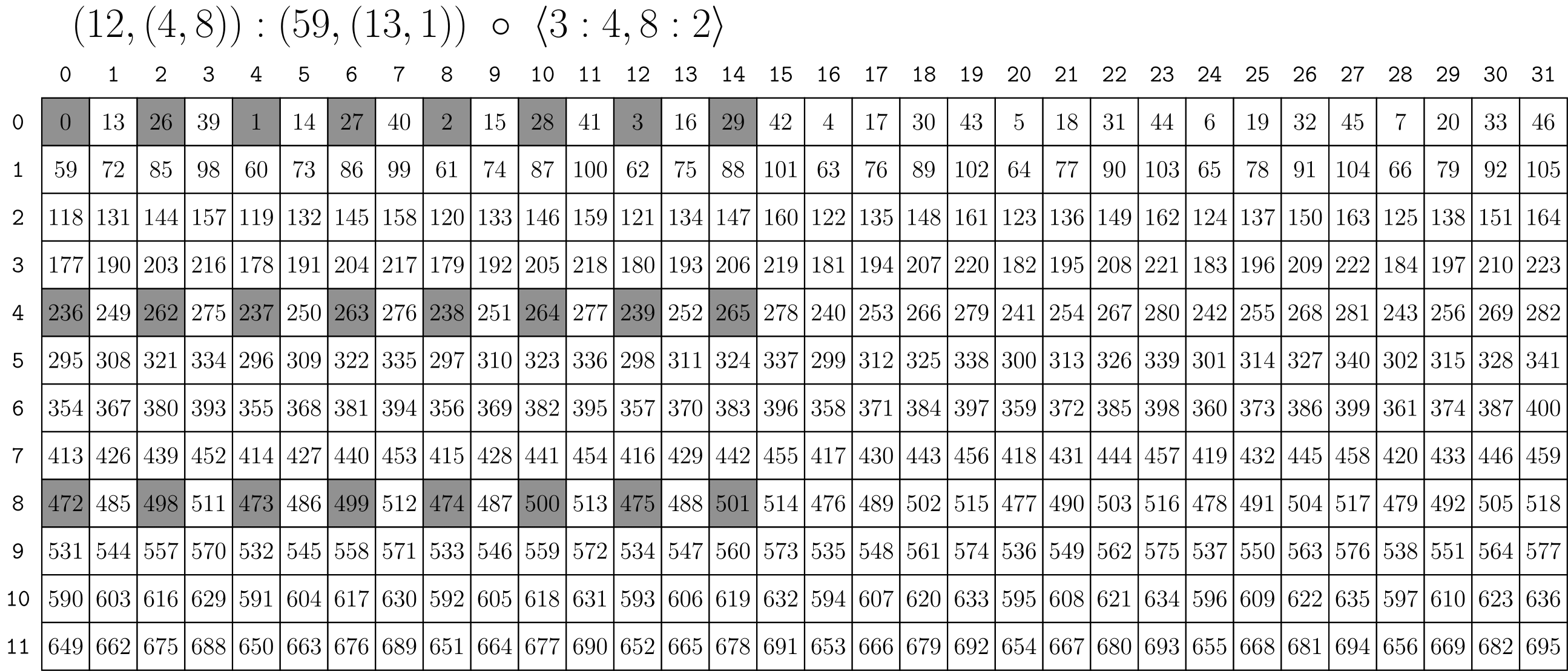
Extract Subtile
// (12,(4,8)):(59,(13,1))
auto a = make_layout(make_shape (12,make_shape ( 4,8)),
                     make_stride(59,make_stride(13,1)));
// <3:4, 8:2>
auto tiler = make_tile(Layout<_3,_4>{},  // Apply 3:4 to mode-0
                       Layout<_8,_2>{}); // Apply 8:2 to mode-1

// (_3,(2,4)):(236,(26,1))
auto result = composition(a, tiler);
结果如下:
2.2.3. 1-D Index 以及 Composition 验证
Layout A (6,2):(8,2):
       0    1
    +----+----+
 0  |  0 |  2 |
    +----+----+
 1  |  8 | 10 |
    +----+----+
 2  | 16 | 18 |
    +----+----+
 3  | 24 | 26 |
    +----+----+
 4  | 32 | 34 |
    +----+----+
 5  | 40 | 42 |
    +----+----+
Layout B (4,3):(3,1):
      0    1    2
    +----+----+----+
 0  |  0 |  1 |  2 |
    +----+----+----+
 1  |  3 |  4 |  5 |
    +----+----+----+
 2  |  6 |  7 |  8 |
    +----+----+----+
 3  |  9 | 10 | 11 |
    +----+----+----+
Composed Layout C:
      0    1    2
    +----+----+----+
 0  |  0 |  1 |  2 |
    +----+----+----+
 1  |  3 |  4 |  5 |
    +----+----+----+
 2  |  6 |  7 |  8 |
    +----+----+----+
 3  |  9 | 10 | 11 |
    +----+----+----+
验证代码:
import cutlass
from cutlass import cute

@cute.jit
def compose_verify():
    A = cute.make_layout((6, 2), stride=(8, 2))
    B = cute.make_layout((4, 3), stride=(3, 1))
    C = cute.composition(A, B)

    flat = cute.coalesce(B)
    for i in cutlass.range_constexpr(cute.size(flat)):
        print(f"C({i}) = {C(i)}, \tflat({i}) = {flat(i)}, \tA(flat({i})) = {A(flat(i))}")


compose_verify()
打印结果:
C(0) = 0,       flat(0) = 0,    A(flat(0)) = 0
C(1) = 24,      flat(1) = 3,    A(flat(1)) = 24
C(2) = 2,       flat(2) = 6,    A(flat(2)) = 2
C(3) = 26,      flat(3) = 9,    A(flat(3)) = 26
C(4) = 8,       flat(4) = 1,    A(flat(4)) = 8
C(5) = 32,      flat(5) = 4,    A(flat(5)) = 32
C(6) = 10,      flat(6) = 7,    A(flat(6)) = 10
C(7) = 34,      flat(7) = 10,   A(flat(7)) = 34
C(8) = 16,      flat(8) = 2,    A(flat(8)) = 16
C(9) = 40,      flat(9) = 5,    A(flat(9)) = 40
C(10) = 18,     flat(10) = 8,   A(flat(10)) = 18
C(11) = 42,     flat(11) = 11,  A(flat(11)) = 42
A. 参考
- CuTe Layout and Tensor Tutorial:deepwiki algegra 使用示例解析
- CuTe Layout Algebra:deepwiki algebra 解析
- cute_layout_algebra.ipynb:官方 CuteDSL notebook
A.1. 学习参考资料
- CuTe Layout Algebra。官方文档
- deepwiki – cutlass – Layout Algebra
- cute Layout 的代数和几何解释。来自知乎 reed 文章
- CuTe Layout and Tensor。来自Yifan Yang (杨轶凡) 博客
- CuTe Layout Representation and Algebra:来自 arxiv 的论文
- CuTe Layout 的范畴论基础
- CuTe 02 - Layout 运算
- Cute概念速通:待阅读
三方学习测试代码:
A.2. 其他资料
- A Generalized Micro-kernel Abstraction for GPU Linear Algebra:NVIDIA PPT
- Algebra – 2.12 Inverses and composition:数学理论:composition
- Categorical Foundations for CuTe Layouts
- Layout Algebra:三方实现的C++ Layout Algebra 库
- On CuTe layouts
A.3. 工具
- 将 SVG 合并到 SVG:工具:合并svg图片
Enjoy Reading This Article?
Here are some more articles you might like to read next: